Export YOLO to ONNX and Run It with ONNX Runtime
ONNX (Open Neural Network Exchange) is a common file format for neural networks. Exporting a trained YOLO model to ONNX lets you run it without PyTorch, on many kinds of hardware, through runtimes such as ONNX Runtime. It is also the usual first step before TensorRT or other accelerators.
This article shows how to export, check and run an ONNX model, and explains the part that trips people up: when you leave the Ultralytics predict function, you must do pre-processing and post-processing yourself.
Why use ONNX
- Smaller runtime. You can deploy with
onnxruntime, OpenCV and NumPy, without installing PyTorch. - Portability. The same file can run on CPU, and with the right execution provider on GPU or other accelerators.
- A common starting point. Many conversion tools (TensorRT, OpenVINO, vendor compilers) accept ONNX.
ONNX is not automatically faster than PyTorch. Whether it helps depends on the model, hardware and runtime settings. Measure it; see measuring FPS and latency correctly.
Step 1: export
With Ultralytics, export is one call:
from ultralytics import YOLO

model = YOLO("best.pt")          # your trained weights
model.export(format="onnx", imgsz=640)
This writes best.onnx next to the weights. A few export options are worth knowing:
imgszsets the input size baked into the graph. Use the same size you trained and validated with.dynamic=Trueallows variable input sizes. It is flexible, but fixed shapes are often simpler and can run better on some runtimes.simplify=Trueruns a graph simplifier. It is commonly on by default for ONNX export, but check the current Ultralytics docs for the defaults in your version.half=Trueexports in FP16, which is only useful on hardware that benefits from it. For CPU use, stay with FP32.
If you are not sure about a flag in your version, check the Ultralytics documentation rather than guessing.
Step 2: inspect the model
Before writing any code, look at what the file expects. Netron, a free model viewer, shows the graph. You can also read the input and output details in Python:
import onnxruntime as ort

sess = ort.InferenceSession("best.onnx", providers=["CPUExecutionProvider"])
inp = sess.get_inputs()[0]
print(inp.name, inp.shape, inp.type)
for out in sess.get_outputs():
    print(out.name, out.shape)
For a standard Ultralytics detection model at 640 input, you typically see an input shaped like [1, 3, 640, 640] and a single output shaped like [1, 4 + number_of_classes, 8400]. The 8400 comes from the three detection scales at 640 input: 80x80, 40x40 and 20x20 grids add up to 8400 candidate predictions. If you change imgsz, this count changes.
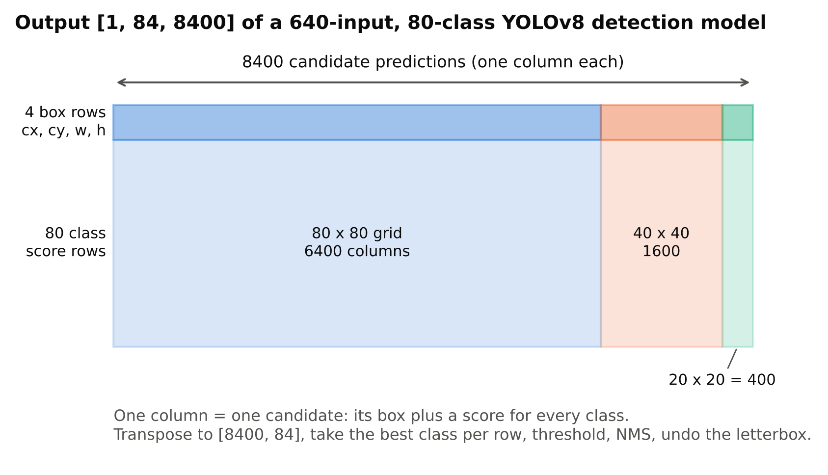
Note that this layout applies to the recent anchor-free Ultralytics detection models. Older YOLOv5 exports differ: they include an objectness value per prediction. Always print your own model's output shape and do not assume.
Step 3: pre-processing
The model expects the same input it saw in training. In Ultralytics, that means:
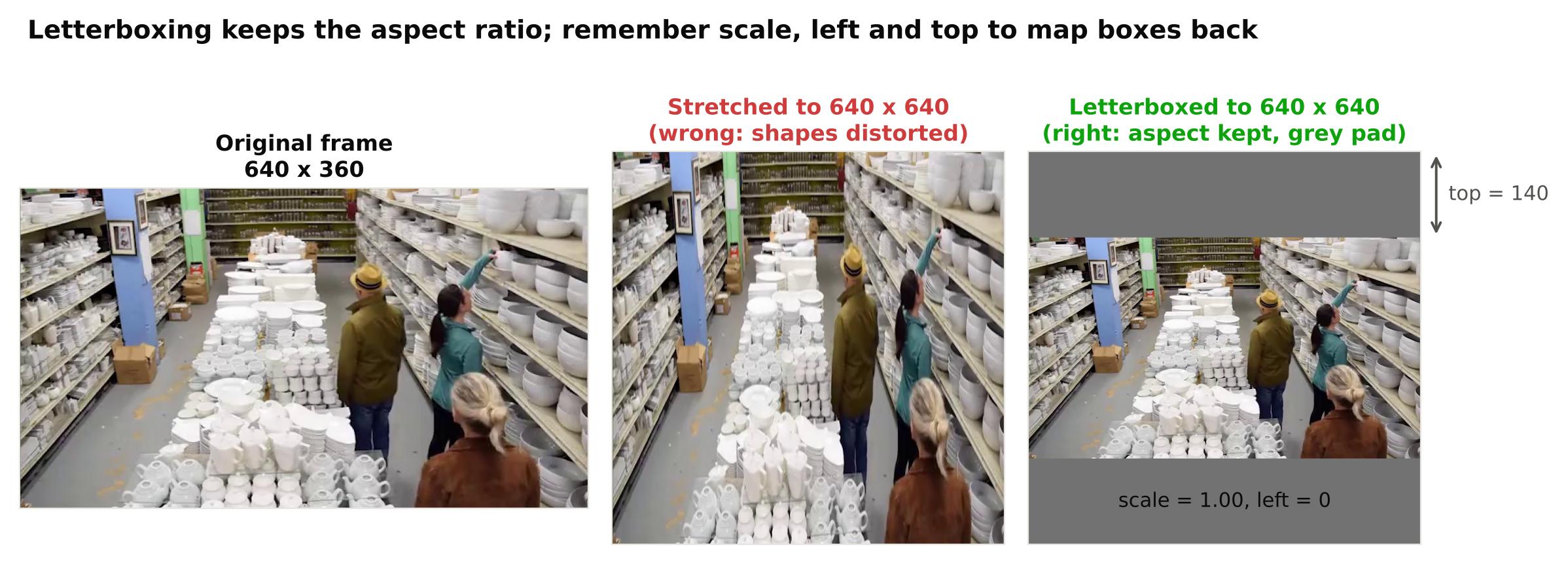
- Letterbox resize. Resize while keeping the aspect ratio, then pad to the square input size. Do not stretch the image.
- Colour order. OpenCV loads images as BGR; the model expects RGB.
- Scale. Divide pixel values by 255 to get floats between 0 and 1.
- Layout. Change from HWC to CHW and add a batch dimension.
A compact version:
import cv2
import numpy as np

def preprocess(img_bgr, size=640):
    h, w = img_bgr.shape[:2]
    scale = min(size / h, size / w)
    nh, nw = int(round(h * scale)), int(round(w * scale))
    resized = cv2.resize(img_bgr, (nw, nh))
    canvas = np.full((size, size, 3), 114, dtype=np.uint8)
    top, left = (size - nh) // 2, (size - nw) // 2
    canvas[top:top + nh, left:left + nw] = resized
    rgb = cv2.cvtColor(canvas, cv2.COLOR_BGR2RGB)
    x = rgb.astype(np.float32) / 255.0
    x = np.transpose(x, (2, 0, 1))[None]
    return x, scale, left, top
The grey padding value of 114 matches the Ultralytics letterbox convention. You must return scale, left and top because you need them to map boxes back to the original image.
Step 4: run inference
x, scale, left, top = preprocess(frame)
outputs = sess.run(None, {inp.name: x})
pred = outputs[0]          # shape [1, 4 + nc, 8400]
Step 5: decode the output
For the anchor-free format, each of the 8400 columns holds four box values followed by one score per class. The box is in centre-x, centre-y, width, height form, in the pixel space of the letterboxed input.
Steps:
- Transpose to
[8400, 4 + nc]. - For each row, take the best class score and its class index.
- Drop rows below your confidence threshold.
- Convert boxes from centre format to corner format.
- Run non-maximum suppression (NMS).
- Undo the letterbox: subtract the padding, divide by the scale, and clip to the image size.
def postprocess(pred, scale, left, top, conf=0.25, iou=0.45):
    p = pred[0].T                       # [8400, 4 + nc]
    scores = p[:, 4:]
    cls = scores.argmax(axis=1)
    conf_all = scores.max(axis=1)
    keep = conf_all >= conf
    p, cls, conf_all = p[keep], cls[keep], conf_all[keep]
    cx, cy, w, h = p[:, 0], p[:, 1], p[:, 2], p[:, 3]
    x1 = (cx - w / 2 - left) / scale
    y1 = (cy - h / 2 - top) / scale
    boxes = np.stack([x1, y1, w / scale, h / scale], axis=1)
    idx = cv2.dnn.NMSBoxes(boxes.tolist(), conf_all.tolist(), conf, iou)
    idx = np.array(idx).reshape(-1)
    return boxes[idx], conf_all[idx], cls[idx]
cv2.dnn.NMSBoxes expects boxes as [x, y, width, height], which is why the code builds them that way. This simple version applies NMS across all classes at once. Ultralytics runs NMS per class by default, so two overlapping boxes of different classes may behave differently. For details on how NMS works and what the thresholds mean, see IoU and NMS explained.
Why results differ from model.predict
If your ONNX output does not match Ultralytics, check these in order:
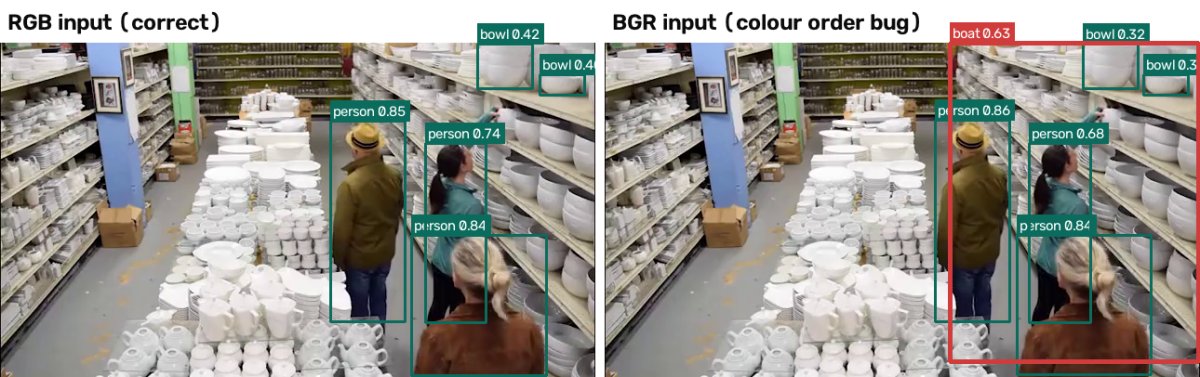
- Wrong colour order. Feeding BGR instead of RGB lowers accuracy without any error message.
- Stretched instead of letterboxed. Boxes will be shifted or the wrong size.
- Missing /255 scaling. Scores collapse.
- Box mapping errors. Forgetting to remove padding or divide by scale.
- Different thresholds. Match the confidence and IoU thresholds you used in the comparison.
- Different input size. The export
imgszmust match what you feed.
A good test: run the same single image through both paths, print the top few detections from each and compare. Small differences in scores are normal; large differences mean a bug.
Validate after export
Do not assume the exported model equals the original. Run your validation set through both and compare metrics. Ultralytics can validate some exported formats directly, but you can also write your own evaluation loop. The point is to confirm accuracy before deployment. mAP, precision and recall explains what to compare.
Performance tips for CPU
- Reduce
imgszif accuracy allows. - Control threads with ONNX Runtime session options, for example
intra_op_num_threads, and test a few values on your hardware. - Keep the Python loop lean. Pre-processing in NumPy can cost as much as inference on a small model.
- Reuse one session. Creating a session per frame is very slow.
- Warm up with a few dummy runs before timing.
Checklist
- Exported with the same
imgszas training and validation. - Input and output shapes printed and understood.
- Letterbox, RGB and /255 applied; boxes mapped back correctly.
- NMS implemented and thresholds matched to your comparison.
- Metrics on a validation set compared with the original model.
- One session reused; warm-up done before timing.
Next steps
Continue with TensorRT for YOLO if you have an NVIDIA GPU, or INT8 Quantization for Detectors to shrink the model further.