Measuring FPS and Latency Correctly
"How fast is it?" sounds like a simple question. In computer vision it rarely is. A single FPS number can mean the model's forward pass, the whole pipeline from camera to alert, or an average over a lucky run. Numbers shared online often leave out which one they mean, and that makes them hard to compare.
This article shows how to measure speed in a way you can trust, using your own model on your own hardware.
Define the terms
- Latency: time for one frame to go from input to result. Measured in milliseconds.
- Throughput (FPS): how many frames per second the system processes over time.
- Model time: time inside the network's forward pass only.
- End-to-end time: everything: capture or decode, pre-processing, inference, post-processing (NMS, tracking) and delivery of results.
These are different. A system can have high throughput and poor latency, for instance when it batches frames or queues them. A model can run in a few milliseconds, while the full pipeline is slower because decoding and Python code dominate.
Decide which number answers your question. If you want to know whether a chosen board can handle your cameras, you need end-to-end throughput. If you want to compare two model sizes, model time is useful, but only if the rest of the setup is identical.
Why naive measurements mislead
No warm-up
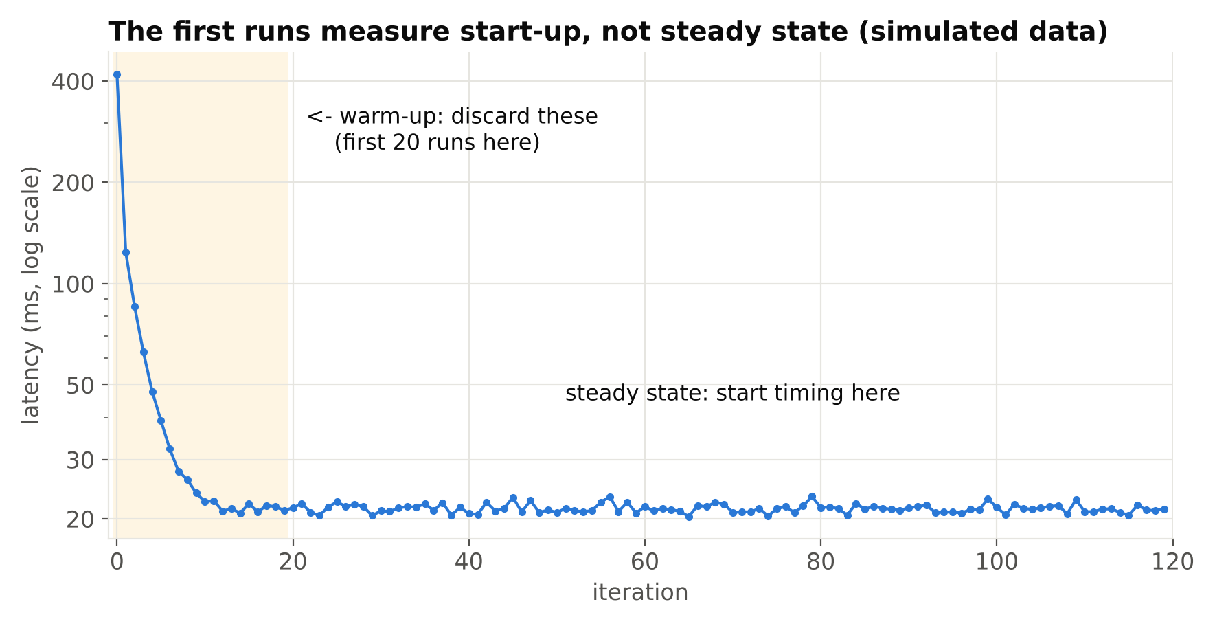
The first inferences are slow. Libraries load kernels, allocate memory, build caches and, on GPUs, initialise contexts. Some runtimes compile or tune on first use. If you time the first few runs, you measure start-up, not steady state.
Fix: run a number of dummy inferences first (ten to fifty is typical), then start timing.
Asynchronous GPU execution
GPU calls are often asynchronous. Your Python code returns before the GPU finishes. If you time with a simple timer around the call, you may measure only the time to queue the work.
In PyTorch, call torch.cuda.synchronize() before reading the end time. Other runtimes have their own ways to wait for completion; fetching the output to the CPU usually forces completion. If you do not synchronise, your results can look impossibly fast.
Wrong timer
Use time.perf_counter() in Python. It is a monotonic, high-resolution clock meant for timing intervals. time.time() can jump and has lower resolution on some systems.
Averaging hides problems
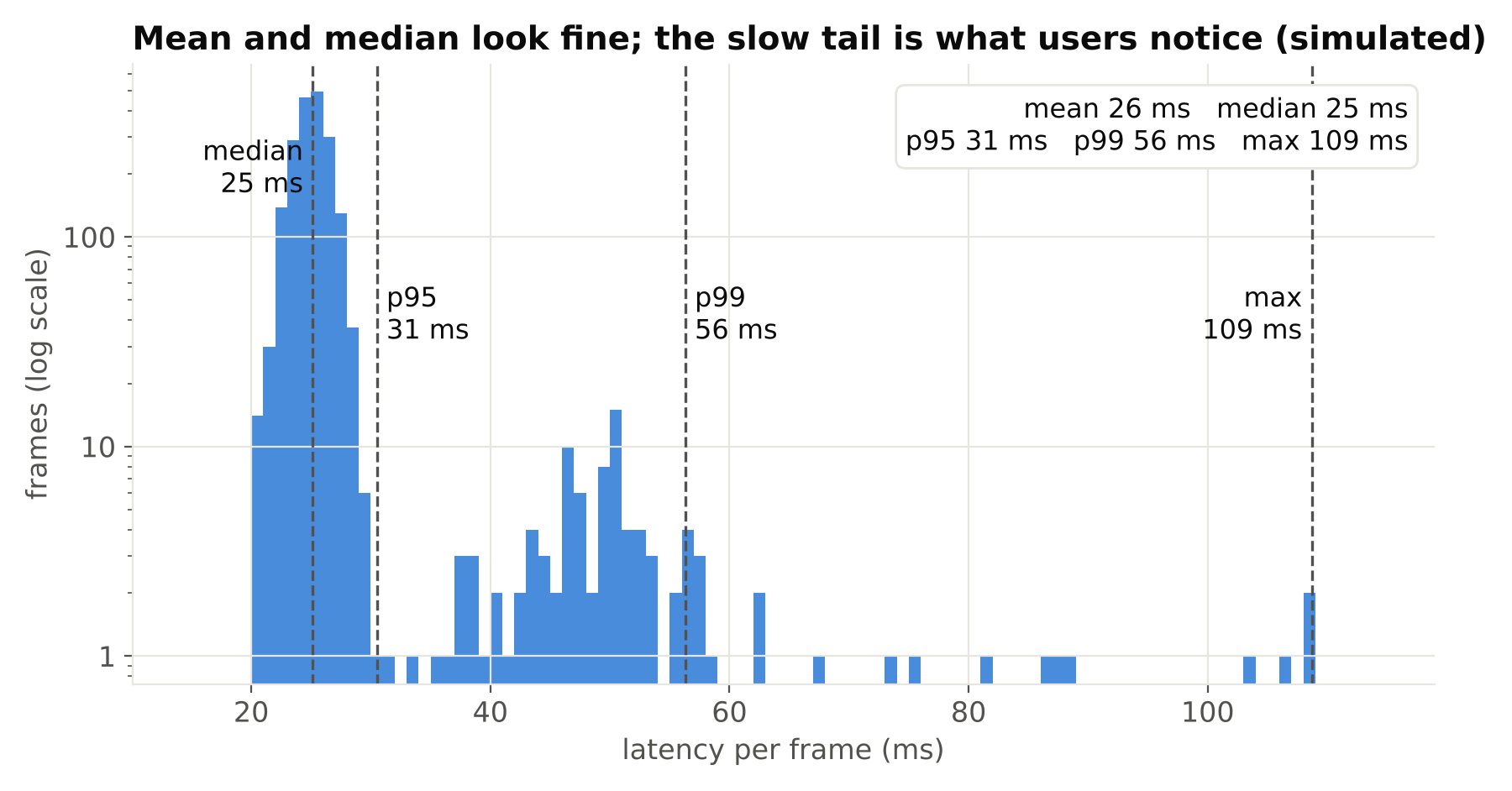
A mean can look fine while the system stutters. Report the median and a high percentile, such as the 95th or 99th, and the worst case. For alerting systems, the slow tail often matters more than the average.
Cold hardware
On small boards, a short test runs while the device is cool. After some minutes, heat can cause throttling and slower speed. Run long enough for temperatures to stabilise. See power, cooling and storage for an edge AI box.
Dynamic clocks and power modes
Many devices change clock speeds based on load and power settings. Record the power mode and note it with your results. A benchmark in one mode is not comparable to another.
A simple benchmark method
Here is a basic template for timing a model function:
import time
import numpy as np

def benchmark(run, warmup=20, iters=200):
    for _ in range(warmup):
        run()
    times = []
    for _ in range(iters):
        t0 = time.perf_counter()
        run()
        times.append((time.perf_counter() - t0) * 1000.0)
    t = np.array(times)
    return {
        "median_ms": float(np.median(t)),
        "p95_ms": float(np.percentile(t, 95)),
        "max_ms": float(t.max()),
    }
Here run is a function that performs the step you care about. For a GPU model, make sure run includes synchronisation or retrieval of results. Pass a real image, or a real frame, not a tensor of zeros, because input content rarely changes speed for a fixed network but can for post-processing (the number of boxes affects NMS time).
Repeat the test several times, on separate runs of the program, to see how much results vary.
Split the pipeline into stages
To find the bottleneck, time each stage separately:
- Capture or decode: reading and decoding the frame.
- Pre-processing: resize, colour conversion, normalisation.
- Inference: the forward pass.
- Post-processing: decode outputs, NMS, tracking, rules.
Ultralytics results include a speed dictionary with pre-process, inference and post-process times in milliseconds for each prediction. That is a convenient start for model-level timing, but it does not include video decoding or your own application code, so time those yourself.
With stage timings, you often find surprises. A common one: the model takes a few milliseconds, while pre-processing in NumPy or decoding a high-resolution stream takes longer. Optimising the network would then bring little gain. See reading RTSP streams with OpenCV and FFmpeg for stream-related delays.
Batch size effects
Batching groups several frames into one forward pass. On GPUs it usually raises throughput because the hardware is used more fully. But it also raises latency: the first frame waits until the batch fills, and the whole batch finishes together.
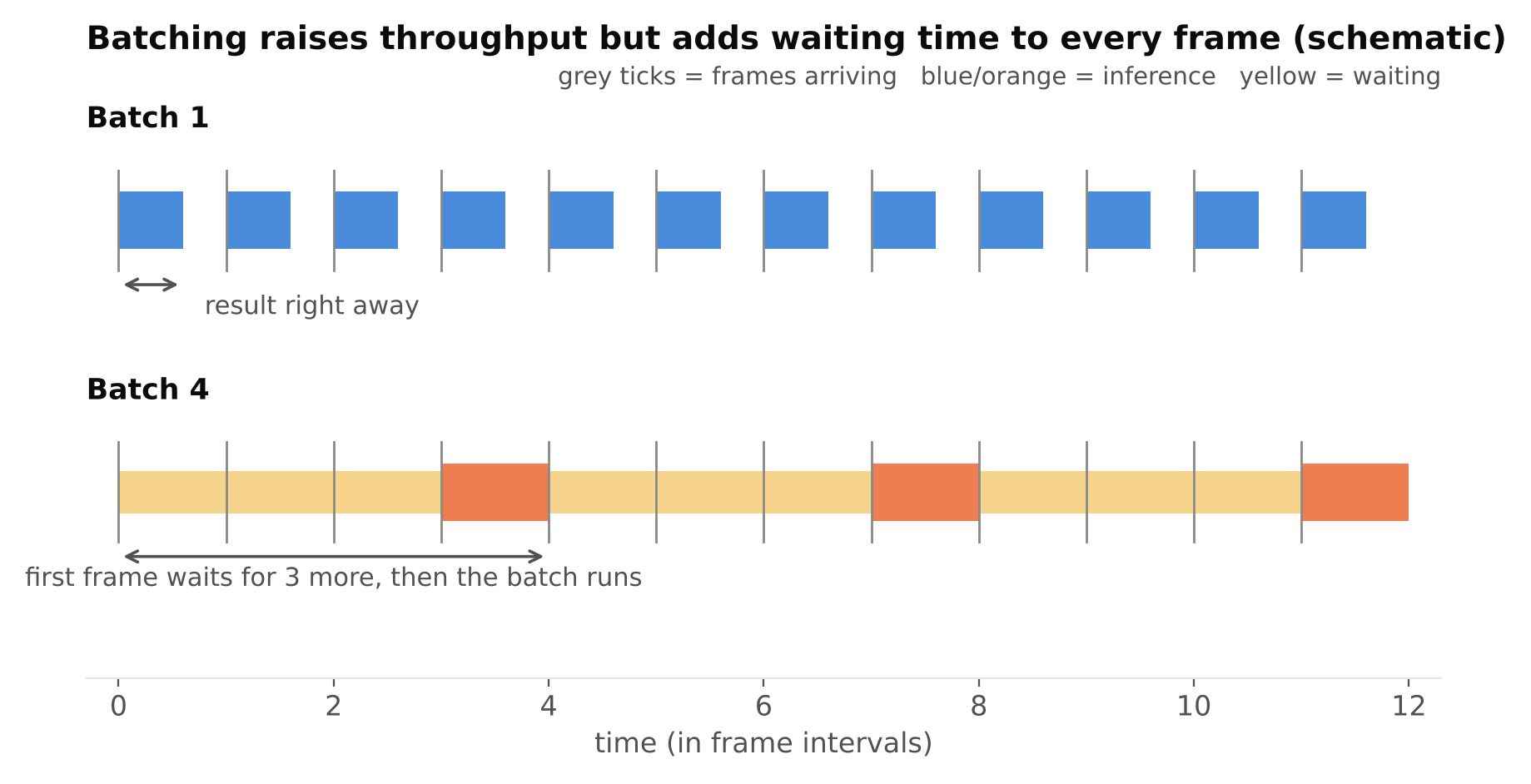
So report batch size with every number. A result of "X FPS at batch 8" and one at batch 1 answer different questions. For a single live camera where fast alerts matter, batch 1 reflects reality. For processing many streams on one GPU, a larger batch may be right. Scaling decisions are discussed in scaling video analytics to hundreds of camera streams.
Measure under realistic conditions
- Use real input. The same resolution, codec and content as production.
- Include all streams. Run the number of concurrent cameras you plan to support. Streams compete for CPU, memory and bandwidth.
- Run long enough. At least until temperature and memory use have levelled off. For stability, a multi-hour test is better.
- Watch resources. Log CPU, GPU use, memory and temperature during the test. A pipeline that hits full CPU will drop frames under extra load.
- Check dropped frames. If a camera produces frames faster than you process them, something has to drop them or they queue up and latency grows. Know which of these your system does.
Camera-to-alert latency
Sometimes you care about real wall-clock delay: from the event in the scene to the alert reaching a person. This includes camera encoding, network, buffering, decoding, analysis, rules and notification delivery. You cannot see all of it from inside your code.
One approach: show a clock or a visible change in front of the camera and compare when the alert fires. This is crude but honest. Also check buffers in your capture library, since a growing buffer can add seconds of delay without any change in measured FPS.
Report results properly
When you share or record a benchmark, include:
- Hardware, power mode and cooling.
- Software versions: framework, runtime, drivers.
- Model name, input size, precision (FP32, FP16, INT8) and export format.
- Batch size.
- What was timed: model only or end-to-end.
- Number of warm-up and measured iterations.
- Median and high percentile, not only the mean.
Without these, a number cannot be reproduced or compared. This also protects you from fooling yourself when you try an optimisation. Change one thing at a time and re-measure.
Common mistakes
- Timing the first run.
- Forgetting GPU synchronisation.
- Quoting model time as if it were system speed.
- Comparing numbers across different input sizes or precisions.
- Using only the mean.
- Testing a cool board for 30 seconds.
- Measuring one stream and claiming support for many.
Checklist
- Decide what you measure: model time, throughput or end-to-end latency.
- Warm up before timing, and use
time.perf_counter(). - Synchronise or fetch results when using a GPU.
- Time each pipeline stage.
- Report median, a high percentile and worst case.
- Record batch size, precision, power mode and versions.
- Test with real footage, real stream counts and a long run.
Next steps
Apply these methods in Raspberry Pi vs Jetson Orin Nano for Object Detection and Scaling Video Analytics to Hundreds of Camera Streams.