How YOLOv7 Gets Real-Time Speed with Re-parameterization
Some models are built one way for training and run another way at inference. Re-parameterization is the trick that makes this possible, and YOLOv7 uses it. The idea is simple once you see it: a model can have a rich, multi-branch structure that helps it learn, then be folded into a plain, fast structure that produces the same outputs. This article explains the idea without heavy maths and covers what it means when you deploy.
I will describe the general technique and how it applies to YOLOv7 at a conceptual level. I will not quote speed or accuracy figures. Those depend on hardware and settings, and you should take them from the official paper and repository, then measure on your own device.
The core problem
During training, a network benefits from extra paths. Parallel branches give gradients more routes, make optimisation easier, and let the model learn features at different kernel sizes. But at inference, branches cost time. Each extra branch means extra memory reads, extra operations and more complex scheduling. On many devices, memory movement matters as much as arithmetic.
So you would like the best of both: a complex structure while learning, a simple one while running. Re-parameterization does that.
The idea in one example
Consider a block that, during training, has three parallel branches:
- a 3x3 convolution,
- a 1x1 convolution,
- an identity shortcut (the input passed straight through).
Their outputs are added together. This structure comes from the RepVGG line of work, which YOLOv7's approach builds on.
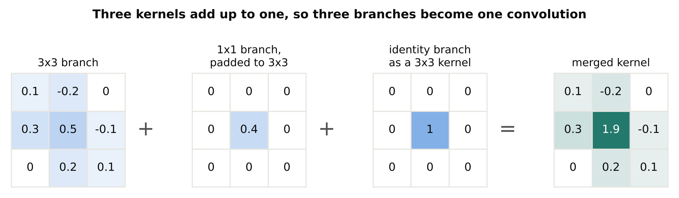
Convolution is a linear operation. Adding the outputs of several linear operations is itself a single linear operation. That means the three branches can be mathematically combined into one 3x3 convolution with different weights:
- The 1x1 kernel is padded with zeros to 3x3 size, so it can be added to the 3x3 kernel.
- The identity branch is equivalent to a 3x3 kernel with a single 1 in the centre (for matching channels), so it can be added too.
- Add the kernels together, and add the biases.
The result is one 3x3 convolution that gives the same output as the three-branch block. Same function, fewer operations, simpler graph.
Batch normalisation gets folded in
Real blocks have batch normalisation (BN) after each convolution. BN is also a fixed linear operation at inference: it scales and shifts each channel using statistics learned during training. Because it is linear, you can fold it into the preceding convolution by adjusting that convolution's weights and bias.
So the conversion has two stages: fold BN into each branch, then merge the branches into one kernel. After that the inference graph contains plain convolutions, and activations in between.
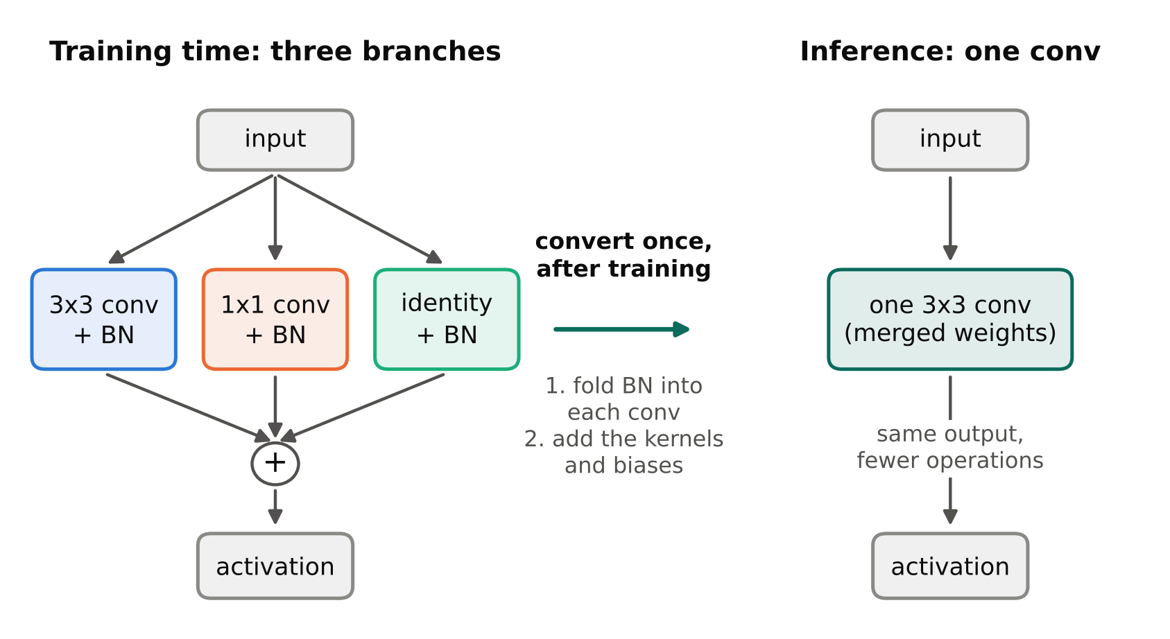
An important detail: this works at inference because BN uses its stored running statistics. During training, BN uses batch statistics, so the fusion is only valid for the trained, frozen model. You do not merge before training ends.
What YOLOv7 does
YOLOv7's paper describes a set of training techniques it calls a "trainable bag of freebies", and planned re-parameterized convolution is one of them. The authors observed that simply dropping the RepVGG-style identity connection into every place does not always work, especially where the block already sits inside a residual or concatenation structure, since the identity would conflict with the existing shortcut. So they plan where re-parameterization is applied and use a variant of the block without the identity branch in places where an identity path already exists.
I am describing this from the paper's general argument. If you need the exact block layout, read the paper and the model configuration files in the repository, rather than relying on a blog summary.
What this means for you
Training and inference models differ
A YOLOv7 checkpoint straight out of training holds the multi-branch structure. To get the fast version, the weights are converted, producing a deployed model with merged layers. The official repository provides a way to do this conversion; follow its instructions for the exact script and steps.
Practical consequences:
- Speed measurements must use the converted model. Benchmarking the training-time structure and quoting it as inference speed gives a misleading result.
- File size and parameter counts change. The merged model has fewer parameters and layers than the training model. Be careful when comparing numbers from different sources, because some report one and some the other.
- The merge is not reversible in a useful way. Keep the original training checkpoint if you may want to fine-tune again.
Exporting to ONNX or TensorRT
If you export a model for deployment, make sure you export the re-parameterized version. Exporting the training graph produces a larger, slower file for no reason. After conversion, validate that outputs match: run the same images through the original and converted models and compare detections. They should match closely. Tiny numerical differences from floating-point arithmetic are normal. Large differences mean the conversion went wrong.
If your tools handle BN folding on their own (many export and optimisation tools fuse convolution and BN automatically), that overlaps with part of this work, but it does not replace the branch merging, which is specific to the model structure.
Quantisation
Merged kernels can have a different range of values than the individual branches. When quantising to INT8, this can affect how well the model tolerates reduced precision, and some re-parameterized designs are known to need care here. Always measure accuracy after quantisation on a representative set rather than assuming it is fine. See INT8 Quantization for Detectors.
Why the trick works for speed
Speed on real hardware depends on more than counting operations. A single large convolution is typically friendlier to GPUs and accelerators than several small branches followed by additions, since it reduces memory traffic and kernel launches. That is the mechanism behind the benefit. How big the gain is depends on your device and runtime, so test it.
Licence reminder
YOLOv7 is released under GPL-3.0. Its obligations differ from AGPL-3.0, which is used by the Ultralytics models, and both affect commercial use. Check the current licence in the repository and read YOLO Licenses Explained. This is not legal advice.
A simple way to verify a conversion
- Pick 20 or so representative images, including hard ones.
- Run the training-time model and the converted model with the same thresholds.
- Compare boxes, classes and scores. Scores should be nearly identical.
- Time the converted model on the target device using the method in Measuring FPS and Latency Correctly.
- Run your normal validation on the converted model, not just the original.
Common mistakes
- Benchmarking the wrong graph. Measure the converted model.
- Skipping the output comparison. A silent conversion bug can reduce accuracy without any error.
- Deleting the training checkpoint. You may need it for more training.
- Assuming all frameworks do this for you. Check how your pipeline handles it.
- Quoting paper speeds for your device. Paper numbers come from specific hardware and settings.
Key points
- Re-parameterization trains a multi-branch model, then merges the branches into a simpler one for inference.
- It works because convolution and batch normalisation are linear at inference, so their weights can be combined.
- YOLOv7 plans where to use it, avoiding the identity branch where a shortcut already exists.
- Always deploy and benchmark the converted model, and compare its outputs with the original.
- Check accuracy again after INT8 quantisation.
- YOLOv7 is GPL-3.0. Check the current licence before commercial use.
Next steps: Export YOLO to ONNX and Run It with ONNX Runtime, INT8 Quantization for Detectors and YOLO Licenses Explained.